Evaluate at

Some examples of the evaluate_at functionality

import xarray as xr
import numpy as np
import xemc3
import matplotlib.pyplot as plt

# Matplotlib setup
import setup_plt

Matplotlib is building the font cache; this may take a moment.

# Use local helper function to get some data
from get_data import load_example_data

ds = load_example_data()
# If you want to use your own data use something like
# ds = xemc3.load.all("path/to/mydata/")
# or if you have converted it already to a netcdf file
# ds = xr.open_dataset("path/to/mydata.nc")

Trying to download an example file to ../../example-data/ ...

Cloning into '../../example-data'...
warning: redirecting to https://gitlab.mpcdf.mpg.de/dave/xemc3-data.git/
Updating files:  52% (57/108)

done

Updating files: 100% (108/108), done.

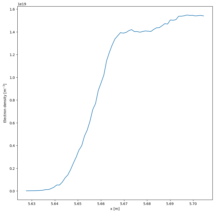
Evaluate along a line of sight

nx = 1000
mapped = ds.emc3.evaluate_at_xyz(
    np.linspace(4.8, 6.0, nx),
    np.linspace(-0.1, 0.1, nx),
    np.linspace(-0.5, 0.5, nx),
    "ne",
    periodicity=5,
    updownsym=True,
    delta_phi=np.pi / 1800,
)
# Add a coordinate
mapped.coords["dim_0"] = np.linspace(4.8, 6.0, nx)
mapped.dim_0.attrs = dict(units="m", long_name="x")

plt.figure()
mapped["ne"].plot()

[<matplotlib.lines.Line2D at 0x782e33bf57f0>]

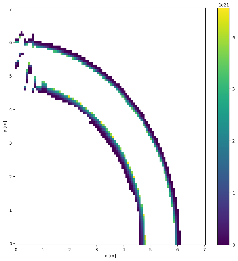
Evaluate along a 2D array

Plotting an \(R\times z\) plane can be done with ds.emc3.plot_rz(key, phi) this allows to plot abitrary cuts of the domain.

# Evaluate an abitrary 2D slice
x = xr.DataArray(np.linspace(0, 7, 100), name="x", dims="x", attrs=dict(units="m"))
y = xr.DataArray(np.linspace(0, 7, 100), name="y", dims="y", attrs=dict(units="m"))
z = 0
# Add coordinates:
x.coords["x"] = x
y.coords["y"] = y


mapped = ds.emc3.evaluate_at_xyz(
    x, y, z, ["ne", "Te"], periodicity=5, updownsym=True, delta_phi=np.pi / 180
)

# Plot the pressure
plt.figure()
(mapped.ne * mapped.Te).plot(x="x", y="y")

<matplotlib.collections.QuadMesh at 0x782e33142c90>

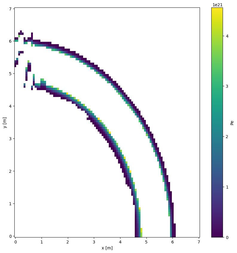
Precalculate the mapping

Rather then directly evaluating a quantity, we can also calculate the mapping first. This is usefull if the same mapping is needed for different simulations, as long as they use the identical grid.

# Evaluate an abitrary 2D slice
x = xr.DataArray(np.linspace(0, 7, 100), name="x", dims="x", attrs=dict(units="m"))
y = xr.DataArray(np.linspace(0, 7, 100), name="y", dims="y", attrs=dict(units="m"))
z = 0
# Add coordinates:
x.coords["x"] = x
y.coords["y"] = y

# We don't pass in the key we want to evaluate
# In this case we get a dataset with indices
mapped = ds.emc3.evaluate_at_xyz(
    x, y, z, key=None, periodicity=5, updownsym=True, delta_phi=np.pi / 180
)

# This time we calculate the pressure
ds["Pe"] = ds.Te * ds.ne
# And then we evaluate with the pre-evaluated indices the pressure in the plane
plt.figure()
ds["Pe"].isel(**mapped).plot(x="x", y="y")

<matplotlib.collections.QuadMesh at 0x782e33c314c0>

Evaluate along a field line

xemc3 doesn’t support field-line tracing

We can however use the webservices, if we are on the IPP network

Warning

Please note that if you don’t use the same magnetic configuration in the fieldlinetracer and the simulations, you might get slightly wrong results or completely wrong results.

Especially, conclusion drawn might be completely wrong!

Always double check the magnetic configurations!