Introduction to xemc3¶

xemc3 is a library for reading the output fron EMC3 simulations into the xarray format.

[1]:

import xarray as xr
import numpy as np
import matplotlib.pyplot as plt
import xemc3

# Matplotlib setup
import setup_plt

Quick introduction to xarray¶

This is just to get a quick introduction of the structure of the xarray data type.

In the cell below we generate a xarray with dimensions \((3,3)\) for variable \(x\) with coordinates \((10,20)\) and \(y\) with coordinates \((1,2,3)\).

[2]:

data = xr.DataArray(
    np.random.rand(2, 3), dims=("x", "y"), coords={"x": [10, 20], "y": [1, 2, 3]}
)
data

[2]:

<xarray.DataArray (x: 2, y: 3)> Size: 48B
array([[0.01622405, 0.50389661, 0.5155113 ],
       [0.34530081, 0.55941462, 0.80778558]])
Coordinates:
  * x        (x) int64 16B 10 20
  * y        (y) int64 24B 1 2 3

data.values¶

Returns the wrapped numpy array, in this case the return value of np.random.rand(2, 3)

[3]:

data.values

[3]:

array([[0.01622405, 0.50389661, 0.5155113 ],
       [0.34530081, 0.55941462, 0.80778558]])

data.dims¶

Returns the name of the dimensions.

[4]:

data.dims

[4]:

('x', 'y')

data.coords¶

Returns the coordinates for all axis directions with coordinate names and datatype of the coordinates.

[5]:

data.coords

[5]:

Coordinates:
  * x        (x) int64 16B 10 20
  * y        (y) int64 24B 1 2 3

data.attrs¶

Returns other attributes in form of a dictionary with you can easily add by generating a new value associated with a new key.

[6]:

data.attrs["units"] = "m"
data.attrs

[6]:

{'units': 'm'}

More on xarray:¶

EMC3 data¶

The prerequisite for this example to work is to have downloaded the file emc3_example.nc and have the libraries specified in this script installed in your enviroment. We recommend using netCDF4 for opening .nc files. The emc3_example.nc can be found and downloaded here: https://gitlab.mpcdf.mpg.de/dave/xemc3-data given that you have acces.

The path specified in the string in the cell below is where you have stored the emc3_example.nc locally on your computer.

[7]:

# Use local helper function to get some data
from get_data import load_example_data

ds = load_example_data()
# If you want to use your own data use something like
# ds = xemc3.load.all("path/to/mydata/")
# or if you have converted it already to a netcdf file
# ds = xr.open_dataset("path/to/mydata.nc")

ds

dataset (ds) explanation¶

When running the codeline ds on the last line of a cell you get an overview of what the xarray object consist of.

ds.coords[‘R_bounds’]¶

R_bounds represents the coordinates of the vertices at the gridcells in the radial direction in the \(xy\)-plane. with \(R = \sqrt{x^2 + y^2}\).

ds.coords[‘z_bounds’]¶

z_bounds represents the coordinates of the vertices of the gridcells in the \(z\)-direction.

ds.coords[‘phi_bounds’]¶

phi_bounds represents the coordinates of the vertices of the gridcells in the \(\phi\)-direction.

[8]:

# The shape is 6 dimensional, as we include 3 dimensions for the vertices
ds.coords["R_bounds"].shape

[8]:

(139, 512, 36, 2, 2, 2)

[9]:

# Note that units are m - xemc3 prefers SI, with only eV as exception
ds.coords["z_bounds"]

[9]:

<xarray.DataArray 'z_bounds' (r: 139, theta: 512, phi: 36, delta_r: 2,
                              delta_theta: 2, delta_phi: 2)> Size: 164MB
[20496384 values with dtype=float64]
Coordinates:
    R_bounds    (r, theta, phi, delta_r, delta_theta, delta_phi) float64 164MB ...
    z_bounds    (r, theta, phi, delta_r, delta_theta, delta_phi) float64 164MB ...
    phi_bounds  (phi, delta_phi) float64 576B ...
Dimensions without coordinates: r, theta, phi, delta_r, delta_theta, delta_phi
Attributes:
    xemc3_type:  geom
    units:       m

Toroidal slice¶

A toroidal slice is defined as the grid of \((R,z)\)-values at a fixed angle \(\phi\). The values of the \(\phi\)-angles used in the W7X grid can be found in the paragraph below and demonstrated in the next cell.

ds.coords[‘phi_bounds’]¶

Running the cell below gives you an array of the \(\phi\) angles.

[10]:

ds.coords["phi_bounds"]

[10]:

<xarray.DataArray 'phi_bounds' (phi: 36, delta_phi: 2)> Size: 576B
[72 values with dtype=float64]
Coordinates:
    phi_bounds  (phi, delta_phi) float64 576B ...
Dimensions without coordinates: phi, delta_phi
Attributes:
    xemc3_type:  geom
    units:       radian

ds.emc3.plot_rz(key, phi = \(\phi\))¶

The key is given as a string, None can be passed as a key if you want to plot the mesh. An example is the angle phi \(= \phi\) which is the angle given in radians as float.

For this particular example(.nc file) the floats of the angle \(\phi\) can be found in the dictionary defined by ds.coords[‘phi_bounds’] which has 2 dimensions; one for either side of the cell for a given angle \(\phi\). There are 37 different values for \(\phi\) since W7-X has a five-fold symmetry which is divided in two up-down symmetric parts and we use a resolution \(1^{\circ}\).

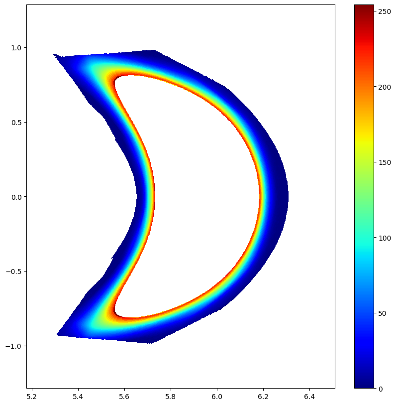
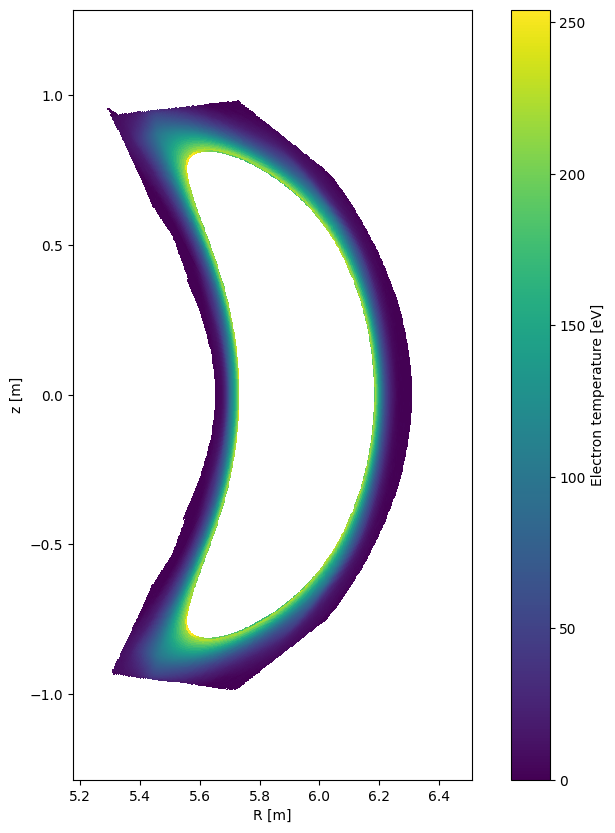
In the cells below are some examples of the parameter electron temperature \(T_e\) plotted in toroidal slices for phi index \(n_{\phi} = [0,18,35]\).

[11]:

# the parameter can be plotted by a one-liner
plt.figure()
ds.emc3.plot_rz("Te", phi=0)

[11]:

<matplotlib.collections.QuadMesh at 0x79cca8250710>

../_images/examples_introduction_21_1.png

[12]:

# for several angles and control
import ipywidgets as widgets

fig = plt.figure()


def plot_Te(ip):
    fig.clear()
    ds.emc3.plot_rz("Te", phi=ip)


ip = widgets.FloatSlider(min=0, max=np.pi / 5, value=0, step=0.01)
widgets.interact(plot_Te, ip=ip)

[12]:

<function __main__.plot_Te(ip)>

../_images/examples_introduction_22_2.png

Simplifying of grid structure¶

The parameter values are defined in each grid cell, but the center or the mean of the vertices of the gridcell: \(\mathbf{r}_{param} = \langle \mathbf{r}_{vertex} \rangle\). A simplified analogy is the centerpoint of a 3D cube.

You can get the center coordinates ds.<direction>_bounds.mean(dim=("delta_r", "delta_theta", "delta_phi"), ignore_missing=True) by averaging over the delta_* dimensions of the variable, as that contains the cell extend in each direction.

[13]:

R = ds.R_bounds.mean(dim=("delta_r", "delta_theta", "delta_phi"))
z = ds.z_bounds.mean(dim=("delta_r", "delta_theta", "delta_phi"))
phi = ds.phi_bounds.mean(dim="delta_phi")
x = R * np.cos(phi)
y = R * np.sin(phi)
x, ds.Te

[13]:

(<xarray.DataArray (r: 139, theta: 512, phi: 36)> Size: 20MB
 array([[[5.90687195, 5.90143282, 5.89057613, ..., 4.27387008,
          4.21925933, 4.16544375],
         [5.90692225, 5.90157835, 5.89081476, ..., 4.27443602,
          4.21980501, 4.16596973],
         [5.90697495, 5.90172636, 5.89105602, ..., 4.27501305,
          4.22036168, 4.16650662],
         ...,
         [5.90673533, 5.90101113, 5.88987631, ..., 4.27223898,
          4.2176884 , 4.1639313 ],
         [5.90677846, 5.90114916, 5.89010684, ..., 4.27277148,
          4.21820095, 4.16442445],
         [5.90682402, 5.90128975, 5.89034014, ..., 4.27331521,
          4.21872462, 4.16492863]],

        [[5.88039947, 5.87478717, 5.86353702, ..., 4.22636359,
          4.17204559, 4.11853643],
         [5.88048206, 5.87503477, 5.86394578, ..., 4.22725027,
          4.17290028, 4.11936057],
         [5.88056438, 5.87528231, 5.86435491, ..., 4.22815464,
          4.17377244, 4.12020195],
 ...
         [5.64755073, 5.63505485, 5.61354696, ..., 3.81421366,
          3.76543708, 3.71779086],
         [5.64922161, 5.63819013, 5.61807245, ..., 3.81753395,
          3.76870465, 3.7210289 ],
         [5.65069075, 5.64113616, 5.6224387 , ..., 3.82111107,
          3.77222496, 3.7245137 ]],

        [[5.59414493, 5.58958172, 5.57387846, ..., 3.75650956,
          3.70552132, 3.65647075],
         [5.59422224, 5.59117652, 5.57709579, ..., 3.76073063,
          3.70983664, 3.66088151],
         [5.59408138, 5.5925006 , 5.5799317 , ..., 3.76497918,
          3.71417615, 3.66525302],
         ...,
         [5.59027424, 5.58100907, 5.56053413, ..., 3.7435559 ,
          3.69303175, 3.64369176],
         [5.59192682, 5.58422348, 5.56529866, ..., 3.74788951,
          3.69714638, 3.64790418],
         [5.59337562, 5.58724114, 5.56988255, ..., 3.75223099,
          3.701277  , 3.65213093]]], shape=(139, 512, 36))
 Dimensions without coordinates: r, theta, phi
 Attributes:
     xemc3_type:  geom,
 <xarray.DataArray 'Te' (r: 139, theta: 512, phi: 36)> Size: 20MB
 array([[[    nan,     nan, ...,     nan,     nan],
         [    nan,     nan, ...,     nan,     nan],
         ...,
         [    nan,     nan, ...,     nan,     nan],
         [    nan,     nan, ...,     nan,     nan]],

        [[    nan,     nan, ...,     nan,     nan],
         [    nan,     nan, ...,     nan,     nan],
         ...,
         [    nan,     nan, ...,     nan,     nan],
         [    nan,     nan, ...,     nan,     nan]],

        ...,

        [[1.1342 , 1.1342 , ..., 0.50556, 0.50556],
         [1.0876 , 1.0876 , ..., 0.43205, 0.43205],
         ...,
         [0.90547, 0.90547, ..., 0.59837, 0.59837],
         [0.99312, 0.99312, ..., 1.4215 , 1.4215 ]],

        [[    nan,     nan, ...,     nan,     nan],
         [    nan,     nan, ...,     nan,     nan],
         ...,
         [    nan,     nan, ...,     nan,     nan],
         [    nan,     nan, ...,     nan,     nan]]], shape=(139, 512, 36))
 Dimensions without coordinates: r, theta, phi
 Attributes:
     xemc3_type:  mapped
     long_name:   Electron temperature
     units:       eV)

Use of NaN values in xEMC3¶

Not all gridcells have a defined parameter value attached to it. This is mostly the outer and inner region of the grid where the values of many parameter has been ignored because in the specific regions the quantity is not evolved. This is illustrated in the above plot example of the electron temperature \(T_e\). In the cell below you can see how large a fraction of the total number of gridpoints the mesh for the electron temperature that has NaN as a value.

[14]:

n_nans_Te = np.sum(np.isnan(ds.Te)).data
print("How many nans in Te field?", n_nans_Te)
print(
    f"Fraction of nans with respect to gridcells: {n_nans_Te / ds.Te.size * 100:.2f} %"
)

How many nans in Te field? 584972
Fraction of nans with respect to gridcells: 22.83 %

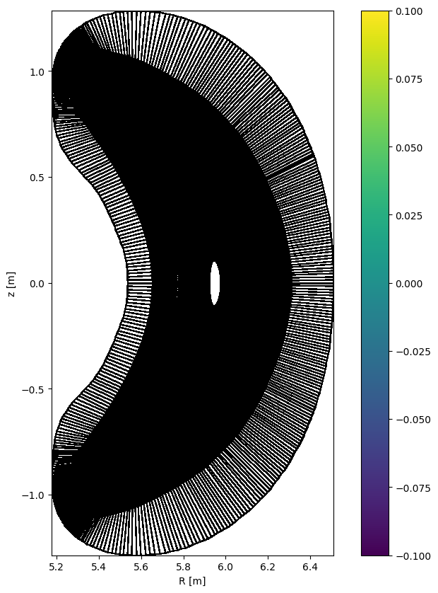
Grid¶

In the cell below there is an interactive plot of the grid. You can use the slider to iterate through all toroidal slices(all \(\phi\) angles).

[15]:

import ipywidgets

fig = plt.figure()

def plot_emc3grid(ip):
    fig.clear()
    ds.emc3.plot_rz(None, phi=ip)

ip = ipywidgets.FloatSlider(min=0, max=np.pi / 5, value=0, step=0.01)
ipywidgets.interact(plot_emc3grid, ip=ip)

[15]:

<function __main__.plot_emc3grid(ip)>

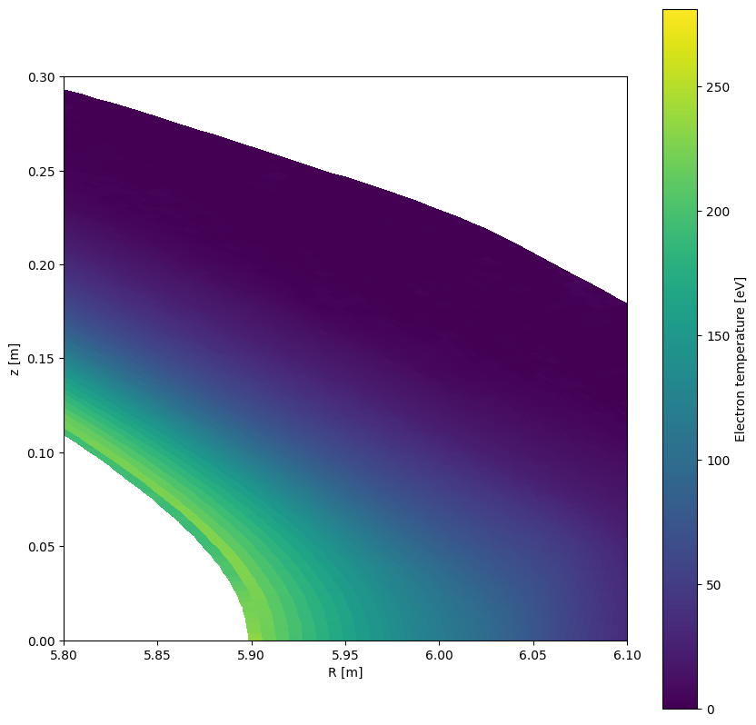
../_images/examples_introduction_28_2.png

Grid with boundaries¶

Interactive plot of the grid, here you can use the ipywidget slider to iterate through all toroidal slices, the rmin and rmax to set the boundaries in r direction, and the zmin and zmax to set the boundaries in z direction.

[16]:

plt.figure()
ds.emc3.plot_rz("Te", phi=np.pi / 5, Rmin=5.8, Rmax=6.1, zmin=0, zmax=0.3)

[16]:

<matplotlib.collections.QuadMesh at 0x79cca7a7ebd0>

../_images/examples_introduction_30_1.png

Periodic boundary conditions for plotting¶

Naturally the data does not have periodic boundary conditions, which means that the last dataframe would be equal to the first. In the case of emc3 data the periodicity is in the theta direction. For plotting the dimension of the theta grid is increased by one and set to the first values in the theta direction. This is for tha plot to “complete the orbit” in the theta direction for it to be closed.

[17]:

fig = plt.figure()


def plot_Te_zoomed(ip):
    fig.clear()
    c = plt.pcolormesh(
        ds.emc3["R_corners"][:, :, ip],
        ds.emc3["z_corners"][:, :, ip],
        ds.Te[:, :, ip],
        cmap=plt.cm.jet,
        shading="auto",
    )
    plt.colorbar(c)


phislider = ipywidgets.IntSlider(min=0, max=35)
ipywidgets.interact(plot_Te_zoomed, ip=phislider)

[17]:

<function __main__.plot_Te_zoomed(ip)>

../_images/examples_introduction_32_2.png

Introduction to xemc3¶

Quick introduction to xarray¶

data.values¶

data.dims¶

data.coords¶

data.attrs¶

More on xarray:¶

EMC3 data¶

dataset (ds) explanation¶

ds.coords[‘R_bounds’]¶

ds.coords[‘z_bounds’]¶

ds.coords[‘phi_bounds’]¶

Toroidal slice¶

ds.coords[‘phi_bounds’]¶

ds.emc3.plot_rz(key, phi = \(\phi\))¶

Simplifying of grid structure¶

Use of NaN values in xEMC3¶

Grid¶

Grid with boundaries¶

Periodic boundary conditions for plotting¶

Table of Contents

Previous topic

Next topic

This Page